Help

Here is an example of how to create a diagram for a version of the famous Mere Addition Paradox and to export it for use in an external program, e.g. a word processor program.

Open a new web browser tab with the diagram editor web page or just click here to do so. All steps in the editor are also illustrated in the two pictures below.

To create the diagram:

1. Set the title to The Mere Addition Paradox.
2. Add two more alternatives by clicking + at the top right of the table.
3. Add three more populations by clicking + at the bottom left of the table.
4. Enter labels for the three alternatives: A, A+, and B.
5. Enter Sizes for the four populations: 20, 20, 20, and 40.
6. Enter the utility numbers 5, 5, 1, and 4.

To export the diagram:

7. Click on Menu to open the menu.
8. Click on Export to open the export dialog.

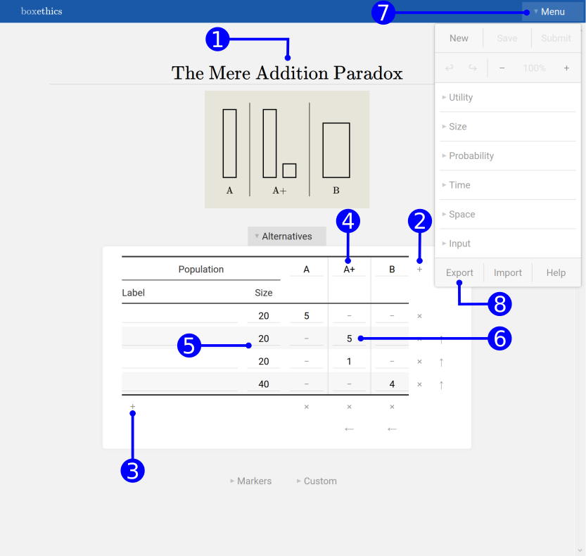
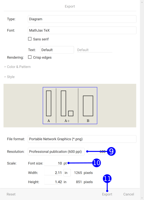
9. Set the Resolution, for example to Professional publication (600 ppi).
10. Set the Font-size used for labels on diagrams in your document, for example to 10 pt.
11. Click Export to download the picture to your computer.

Save the picture to your computer and insert it into your external document.

The ethics of distribution is about the evaluation of alternatives with respect to their distributions of welfare (or opportunity to welfare).

Welfare is what is good for an individual. In the ethics of distribution, it is assumed that, at least in principle in some cases, the welfare levels or quality of life of different individuals can be compared (on a ratio scale and represented by a number, often called utility.

One field of application is public health where QALYs (quality adjusted life years) are measured. Another is the ethics of future generations that is riddled with a number of problems and paradoxes concerning the composition and size of future populations.

A case consist of a number of alternatives with a utility distribution among populations of various sizes.

The information of a case can be arranged in a table. This is how it is entered in the editor.

The information of a case can be arranged in a box-diagram. The height of a box represents the relative utility. The width of a box represents the population size (in atemporal diagrams, see Time). The editor creates diagrams automatically from the information entered into the table.

Click on the diagram to view it in the editor.

Selection

Text input can be started by either selecting a field in the table or an element in the diagram.

Multi line text

Multi line text can be set by using double backslash, \\, or pressing pressing the return key, ↵. For

\(\text{first line}\)
\(\text{second line}\)

enter

first line\\second line

Math

Math input is supported by \(\mathrm{\LaTeX}\) commands. Here is a short List of Mathematical Symbols.

Note: \(\mathrm{\LaTeX}\) has not to be installed to use these commands in the editor and the exported diagrams in other applications.

Math has to be entered in math mode. To enter math mode either bracket with $-signs, like $x$. This can also be accomplished by selecting the text to be put in math mode and pressing $. Alternatively, math mode can be set as primary mode of input, in the Menu Input Math mode, see Settings. In math mode normal, text has to be bracketed in \text{}, like \text{some normal text}. Since $ is used to enter math mode it has to be escaped as \$ to be used as symbol.

Sub- and superscript

Sub- and superscript can be set in math mode using _ and ^, respectively. For more than one character in sub- or superscript use the braces { and }. For \(\text{A$_{23}$}\) enter

A$_{23}$

In this way variables in the subscript will be set as math, for example \(\text{A$_{mn}$}\). For a more uniform rendering either set everything in math mode or set the subscript as in text mode. For example, for \(\text{$A_{mn}$}\) and \(\text{A\(_\text{mn}\)}\) enter, respectively,

$A_{mn}$
A$_\text{mn}$

Alternatively, bracketing text with _{ and } can be accomplished by selecting the text to be set in subscript and pressing _.

Special characters

Special characters can be set by using \(\mathrm{\LaTeX}\) math commands. For example for \(\alpha\) enter $\alpha$

Note: Math can be used in various ways. For example, by combining two \(\approx\), \approx, symbols and a negative space, \!, to $\approx\!\approx$ one gets a wave like symbol \(\approx\!\approx\).

The Mere Addition Paradox

Alternatives are arranged in a table. It is also possible to select items in the table by selection in the diagram.

Label

Enter the label of an alternative at the top row. Click + at the top right to add an alternative.

Distributions

Click × at the bottom under a distribution column to remove a distribution from an alternative.

Probability

To edit probabilities check 'Edit probabilities' in the Settings. Click + next to a probability add a distribution with a probability to an alternative.

The Fairness of Lotteries

Population

Click + at the bottom left to add a population. Click × at the left next to the population row to remove a population.

Population label

Enter the label of a population at the left column.

Population size

Enter the size of a population. Enter > before the size of a population to make it appear larger.

The Repugnant Conclusion

There are some abbreviations for sizes:

• K for 10³ = 1,000
• M for 10⁶ = 1,000,000
• B for 10⁹ = 1,000,000,000
• T for 10¹² = 1,000,000,000,000

For example, 10B for 10,000,000,000.

Utility

Utility box

Enter a numeric utility to set the height of a utility box.

Text

Enter a non-numeric term to make this term appear instead of a utility box.

A spectrum

Note: It is possible to move a label to the negative utility side by using -[label.

Hide

Leave blank to make the population disappear in the distribution.

Dotted utility box

Enter a slash, /, followed a numeric utility to create a dotted utility box.

2/5

Utility comparison

It is possible to create multiple dotted utility boxes by adding further utility numbers preceded by a slash.

Custom utility label

Enter a numeric utility followed by a squared bracket open, [, and a text to create a label for the utility.

100[very\\high\\welfare

Add a marker to indicate a utility level. In alternatives where all populations never-exist no mark will be drawn. However you can force to draw a mark by adding a population and setting its utility to a space,  .

See also Mark 0 utility.

Add custom elements to the diagram. The SVG markup of these elements are added in the text area.

For more details on SVG see the Wikipedia page Scalable Vector Graphics.

There are buttons for simple tools to draw directly onto the diagram:

• Path
• Line
• Rectangle
• Ellipse
• Text

If a tool is selected the draw mode is activated and indicated by a blue box around the diagram which marks the edges of the diagram. To exit draw mode click again on the currently selected tool button or press the Esc key. For every tool there are a number buttons to set attributes, such as fill and stroke color, and text alignment.

The number of attributes and their values that can be set via buttons is very limited. But the SVG markup can be freely changed in the text area. A couple of examples are provided below.

Elements can be drawn with their center at the starting position by pressing the Control key while drawing. Elements can be drawn with equal height and width, e.g. square and circle, by pressing the Shift key while drawing.

Path

Draws a curve from commands in d.

<path d="..." />

Line

Draws a line from the coordinates x1 and y1 to x2 andy2.

<line x1="100" y1="50" x2="40" y2="20" />

Rectangle

Draws a rectangle from the coordinates x and y with dimensions width and height.

<rect x="100" y="50" width="40" height="20" />

Ellipse

Draws an ellipse from the center coordinates cx and cy with radiuses rx and ry.

<ellipse cx="100" cy="50" rx="40" ry="20" />

Text

Draws a text at the coordinates x and y.

<text x="100" y="50">Some text</text>

Group

Groups the embraced elements.

<g>...</g>

Attributes

class

There are a couple of predefined classes that set the attriutes to the same as for automatically created elements in the diagram. For example, class="marker" will set the stroke of an element as for the markers.

• box stroke as for utility boxes
• box2 stroke as for secondary utility boxes
• marker stroke as for marker
• marker0 stroke as for 0 utility marker

Note: Attributes set by a class are superseded by explicitly set attributes, for example those mentioned below.

fill

Sets the fill color. Values can be predefined color names, like fill="orange", and RGB triplets (red, green, blue), like fill="rgb(255,165,0)".

stroke

Sets the stroke color. For values see fill.

stroke-width

Sets the stroke width, like stroke-width=".75".

stroke-dasharray

Sets the stroke pattern of dashes and gaps, like stroke-dasharray="5,5".

text-anchor

Sets the horizontal text alignment, like text-anchor="middle".

dominant-baseline

Sets the vertical text alignment, like dominant-baseline="central".

transform

Transforms the element, like transform="scale(2) translate(20 -40)".

All settings are in the Menu at the top right.

Time

Diagrams can be set to represent the (width of) time (slices) by the width of boxes (instead of the population size).

Timeslices

Enter the number of timeslices for temporal diagrams.

Now

Enter the time of choice, ≥ 0.

The Risky Policy

Scale

Enter a time scale.

Label time

Check to label the timeslices.

Edit time labels

Check to edit the labels of timeslices.

Click on the undo and redo buttons, ↶ and ↷, in the Menu. In some browsers, you can also use the default keyboard shortcuts:

Windows

Undo

Ctrl + Z

Redo

Ctrl + Y or Shift + Ctrl + Z

Mac

Undo

cmd ⌘ + Z

Redo

Shift + cmd ⌘ + Z

Save

To save a diagram click Menu Save. In some browsers, you can also use the keyboard shortcut Ctrl + S.

Fork

To save an already saved diagram under a new filename click Menu Fork. In some browsers, you can also use the keyboard shortcut Ctrl + S.

This will generate a new filename and URL. Save the diagram by saving the URL, for example as a bookmark in your browser.

You can also easily share a diagram with others by sending the URL, for example via copy and paste into an email.

Note: If you ever have forgotten to bookmark a saved diagram you can recover it from your browsing history.

Open the export dialog by clicking on Menu Export.

Almost all application have png- and jpg-file support. So you can work with these formats in any case. Below are some details on the more limited svg-file support.

Inkscape

svg-files can be edited and exported to different file formats by the open SVG graphics editor Inkscape.

• Download Inkscape

Note: The editor combines different elements into groups.

• To select a single element within a group press Ctrl and click on the element.
• To open a group temporarily double click on the group.
• To ungroup a group permanently cick on the group to ungroup and, in the menu, on Object > Ungroup.

\(\mathrm{\LaTeX}\)

\(\mathrm{\LaTeX}\) offers support for vector graphics via Inkscape. There are several methods. With the one described below it is possible to include SVG images and have \(\mathrm{\LaTeX}\) typeset the text.

Export a svg-file for LaTeX:

1. Open the Menu Export dialog.
2. In the Font list select LaTeX export.
3. Click Export to export the svg-file.

Convert a svg-file to a pdf-file in Inkscape:

1. Open the exported svg-file in Inkscape.
2. From the menu select File > Save as....
3. In the File Type list select Portable Document Format (*.pdf).
4. Check PDF+LaTeX: Omit text in PDF, and create LaTeX file.

Insert a pdf-file in LaTeX

Make sure the preamble contains the following.

\usepackage{amsmath} % for enhanced math support
\usepackage{graphicx} % for inclusion of graphics
\usepackage{color} % for text color
\usepackage{grffile} % for larger range of filenames
\usepackage{calc} % for simple arithmetic

Add the figure into the document. For example:

\begin{figure}
  \centering
  \input{"image.pdf_tex"}
\end{figure}

Replace image with the file name.

Putting graphics in separate folder

The default path for graphics is your document folder. If you want to set a different (sub) folder add the following to the preamble:

\graphicspath{{<path>}}

Where you replace <path> by your graphics folder, e.g.

\graphicspath{{images/}}

Scaling the image in LaTeX

To control the size of the image without changing the text size add

\def\svgscale{<scale>}

or

\def\svgwidth{<v-length>}

to the figure. For example:

\begin{figure}
  \centering
  \def\svgscale{.5}
  \input{image.pdf_tex}
\end{figure}

Beware that changing the size of the image without the text can lead to unwanted effects and that the definition is reset for each image.

To control the size of the image including the text size add

\scalebox{<h-scale>}[<v-scale>]{<content>}

or

\resizebox{<h-length>}{<v-length>}{<content>}

to the figure. For example:

\begin{figure}
  \centering
  \scalebox{.5}{\input{image.pdf_tex}}
\end{figure}

Further reading

• How to include an SVG image in LaTeX
• Packages in the ‘graphics’ bundle which is a subset of the graphicx bundle.
• An Improved Environment for Floats which provides option [H] for “put it HERE, period”.

LibreOffice

LibreOffice offers native support for svg-files.

Insert a svg-file in LibreOffice:

• From the menu choose Insert > Image....

This might not always lead to the best results. An alternative is to export to eps-file in Inkscape, see below under Microsoft Word.

Tip: If math input is used in a diagram, e.g. for variables or formulas, then this might be typeset differently from the main text in your document, e.g. in italics. To best imitate this effect use the native Formula functionality to insert variables and formulas.

LyX

LyX offers native support for svg-files.

Insert a svg-file in LyX:

• From the menu choose Insert > File > External Material....
• As Template chose Inkscape figure.

Tip: To have \(\mathrm{\LaTeX}\) typeset the text use the LaTeX export (see \(\mathrm{\LaTeX}\)).

OpenOffice

OpenOffice offers native support for svg-files.

Insert a svg-file in OpenOffice:

• Adding images to a document - Apache OpenOffice Wiki

This might not always lead to the best results. An alternative is to export to eps-file in Inkscape, see above under Microsoft Word.

Further reading

• Adding captions to graphics - Apache OpenOffice Wiki

THE SOFTWARE IS PROVIDED "AS IS", WITHOUT WARRANTY OF ANY KIND, EXPRESS OR IMPLIED, INCLUDING BUT NOT LIMITED TO THE WARRANTIES OF MERCHANTABILITY, FITNESS FOR A PARTICULAR PURPOSE AND NONINFRINGEMENT. IN NO EVENT SHALL THE AUTHORS OR COPYRIGHT HOLDERS BE LIABLE FOR ANY CLAIM, DAMAGES OR OTHER LIABILITY, WHETHER IN AN ACTION OF CONTRACT, TORT OR OTHERWISE, ARISING FROM, OUT OF OR IN CONNECTION WITH THE SOFTWARE OR THE USE OR OTHER DEALINGS IN THE SOFTWARE.